
How VLOOKUP Works
The VLOOKUP function allows you to search for a value in the first column of a specified range and return a value in the same row from another column.
Its syntax is:
=VLOOKUP(lookup_value, table_array, col_index_num, [range_lookup])
Breaking it down:
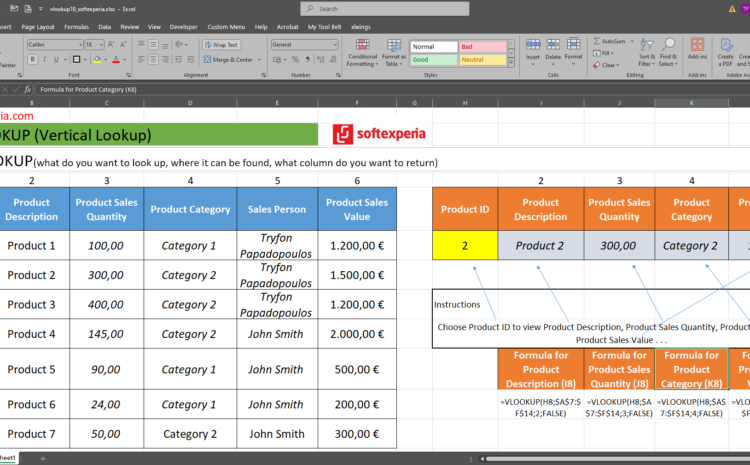
lookup_value: The value you want to look up (e.g., Product ID in cell H8).
table_array: The range where the data is located (e.g., $A$7:$F$14).
col_index_num: The column number in the table from which you want to retrieve data.
[range_lookup]: Use FALSE for an exact match or TRUE for an approximate match.
Example: Retrieving Product Information
Suppose you have a table where:
Column A contains Product IDs,
Column B contains Product Descriptions,
Column C contains Sales Quantities,
Column D contains Product Categories,
Column E contains Sales Persons.
Column F contains Sales Values.
If you enter a Product ID in H8, you can use VLOOKUP to return related information.

Formulas:
Product Description (I8)
=VLOOKUP(H8, $A$7:$F$14, 2, FALSE)
Product Sales Quantity (J8)
=VLOOKUP(H8, $A$7:$F$14, 3, FALSE)
Product Category (K8)
=VLOOKUP(H8, $A$7:$F$14, 4, FALSE)
Product Sales Value (L8)
=VLOOKUP(H8, $A$7:$F$14, 6, FALSE)
Key Points:
=>Ensure that the lookup value (Product ID in H8) exists in the first column of the table range (column A in $A$7:$F$14).
=>Use absolute references ($A$7:$F$14) to prevent the range from shifting if you copy the formula.
=>Set the final argument to FALSE for an exact match.
Download the VLOOKUP example file…
mindstormGR softexperia sales vlookup
Δείτε επίσης